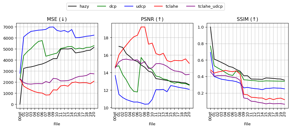
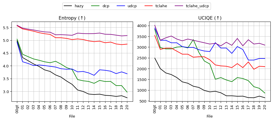
I evaluated output quality on the DeepBlue reference dataset for TCLAHE, DCP, UDCP, and TCLAHE followed by UDCP. I used reference metrics MSE, PSNR, and SSIM, and referenceless metrics entropy and UCIQE. See Figure 2.1.
Figure 2.1: Reference and referenceless Metrics for TCLAHE, DCP, UDCP, and TCLAHE -> UDCP on the DeepBlue dataset. Higher filenames are more turbid. 00gt.png has no turbidity.
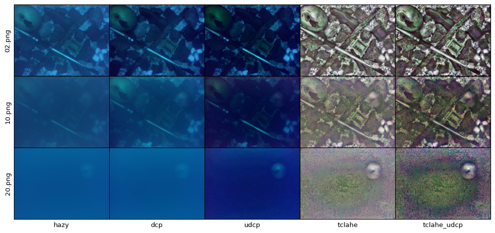
Figure 2.2: Low (02.png), medium (10.png), and high (20.png) turbidity images from the DeepBlue dataset, processed by TCLAHE, DCP, UDCP, and TCLAHE -> UDCP. The hazy column are the original images.
TCLAHE and TCLAHE -> UDCP are consistantly the best performing pipelines (barring their low SSIM scores). DCP seems to modify images the least.
3 Next Steps
Measure runtimes
Add learning pipelines
Choose which Retinex/CLAHE/etc. model-free pipelines to use
Source Code
---title: "Basic metrics"format: html: code-fold: true code-tools: truejupyter: python3author: Benjamin Poulindate: 2025-06-27lightbox: true---I evaluated output quality on the DeepBlue reference dataset for TCLAHE, DCP, UDCP, and TCLAHE followed by UDCP. I used reference metrics MSE, PSNR, and SSIM, and referenceless metrics entropy and UCIQE. See @fig-metrics.```{python}import jsonPRETTY_METRIC_NAMES = {'mse': 'MSE (↓)','psnr': 'PSNR (↑)','ssim': 'SSIM (↑)','entropy': 'Entropy (↑)','uciqe': 'UCIQE (↑)'}REF_METRICS = ('mse', 'psnr', 'ssim')REFLESS_METRICS = ('entropy', 'uciqe')PIPELINES = ('hazy', 'dcp', 'udcp', 'tclahe', 'tclahe_udcp')PIPELINE_COLORS = {'dcp': 'green','udcp': 'blue','tclahe': 'red','tclahe_udcp': 'purple','hazy': 'black'}FILENAMES = ('00gt.png', '01.png', '02.png', '03.png', '04.png', '05.png', '06.png', '07.png', '08.png', '09.png', '10.png', '11.png', '12.png', '13.png', '14.png', '15.png', '16.png', '17.png', '18.png', '19.png', '20.png')FILENAMES_NO_EXTENSION = [filename[:-4] for filename in FILENAMES]ref_data = {}refless_data = {}def make_metric_data(metrics_json, metric_name: str): data = []for pipeline in PIPELINES: data.append([])for filename in FILENAMES: data[-1].append(metrics_json[pipeline][filename][metric])return datawithopen('../data/metrics.json', 'r') as metrics: metrics_json = json.load(metrics)for metric in REF_METRICS: ref_data[metric] = make_metric_data(metrics_json, metric)for metric in REFLESS_METRICS: refless_data[metric] = make_metric_data(metrics_json, metric)``````{python}#| label: fig-metrics#| fig-cap: "Reference and referenceless Metrics for TCLAHE, DCP, UDCP, and TCLAHE -> UDCP on the DeepBlue dataset. Higher filenames are more turbid. `00gt.png` has no turbidity."#| fig-subcap:#| - Reference metrics#| - Referenceless metricsimport matplotlib.pyplot as pltfor metrics, data in ((REF_METRICS, ref_data), (REFLESS_METRICS, refless_data)): fig, axs = plt.subplots(nrows=1, ncols=len(metrics)) axs = axs.flatten()for metric, ax inzip(metrics, axs, strict=True): ax.grid(alpha=0.7) ax.tick_params(axis='x', labelrotation=90) ax.set( xlabel='File',# ylabel=PRETTY_METRIC_NAMES[metric], title=PRETTY_METRIC_NAMES[metric] )for series, label inzip(data[metric], PIPELINES, strict=True): ax.plot( FILENAMES_NO_EXTENSION, series, label=label, color=PIPELINE_COLORS[label] ) handles, labels = axs[0].get_legend_handles_labels() fig.legend(handles, labels, loc='upper center', ncol=len(PIPELINES), bbox_to_anchor=(0.5, 1.1)) fig.set_size_inches(10, 4) fig.tight_layout() plt.show()```See @fig-images for examples of dehazed images.```{python}#| label: fig-images#| fig-cap: "Low (`02.png`), medium (`10.png`), and high (`20.png`) turbidity images from the DeepBlue dataset, processed by TCLAHE, DCP, UDCP, and TCLAHE -> UDCP. The `hazy` column are the original images."from pathlib import Pathimport cv2BASE_PATH = Path('/home/mantis/Documents/ms/underwater-dehazing-toolkit/data/deepblue')FILES = ('02.png', '10.png', '20.png')fig, axs = plt.subplots(nrows=len(FILES), ncols=len(PIPELINES), sharex=True, sharey=True)forfile, axs_row inzip(FILES, axs, strict=True):for pipeline, ax inzip(PIPELINES, axs_row, strict=True): image = cv2.imread(str(BASE_PATH / pipeline /file)) image = cv2.cvtColor(image, cv2.COLOR_BGR2RGB) image_shape = image.shape ax.imshow(image) ax.set_xticks([]) ax.set_yticks([]) ax.set_xticklabels([]) ax.set_yticklabels([]) ax.set( xlabel=pipeline, ylabel=file ) ax.label_outer()fig.subplots_adjust(wspace=0, hspace=0, left=0, right=1, top=1, bottom=0)subplot_width =2subplot_height = (subplot_width / image_shape[1] * image_shape[0])fig.set_size_inches( subplot_width *5, subplot_height *3)plt.show()```TCLAHE and TCLAHE -> UDCP are consistantly the best performing pipelines (barring their low SSIM scores). DCP seems to modify images the least.# Next Steps - Measure runtimes - Add learning pipelines - Choose which Retinex/CLAHE/etc. model-free pipelines to use