Code
import numpy as np
import cv2
import os
import matplotlib.pyplot as plt

TILE_WIDTH = 1280
TILE_HEIGHT = 720

OG_IMGS = (
    "/home/mantis/Documents/ms/data/cup/0.png",
    "/home/mantis/Documents/ms/data/turbid/deepblue/prog/1080/13.jpg",
    "/home/mantis/Documents/ms/data/turbid/milk/prog/1080/19.jpg",
    "/home/mantis/Documents/ms/data/lakes/erie_0/0.png",
    "/home/mantis/Documents/ms/data/lakes/erie_2025_03/frames/blue_1.png",
    "/home/mantis/Documents/ms/data/lakes/erie_2025_07/frames/png/LT_35_100_frame.png",
)

SINGLES_DIR = '/home/mantis/Documents/ms/data/output/summer_end/singles/'
ALGO_DIRS = ('hazy', 'udcp', 'clahe', 'tclahe', 'edn-gtm')

IMAGE_NAMES = ('Cup', 'Deepblue', 'Milk', 'Mr. Crab', 'Erie #1', 'Erie #2')

GRID_WIDTH = len(IMAGE_NAMES)
GRID_HEIGHT = len(ALGO_DIRS)

fig, axes = plt.subplots(GRID_HEIGHT, GRID_WIDTH)

for r, dir in enumerate(ALGO_DIRS):
    if dir == 'hazy':
        image_files = OG_IMGS
    else:
        image_files = sorted([(SINGLES_DIR + dir + '/' + f) for f in os.listdir(SINGLES_DIR + dir) if f.lower().endswith(('.png', '.jpg', '.jpeg'))])
    for c, filepath in enumerate(image_files):
        img = cv2.imread(filepath, cv2.IMREAD_COLOR_RGB)
        if img is None:
            raise FileNotFoundError(f'Could not find {filepath}')
        img = cv2.resize(img, (TILE_WIDTH, TILE_HEIGHT), interpolation=cv2.INTER_LINEAR)

        ax = axes[r, c]
        ax.imshow(img)

        ax.set_xticks([])
        ax.set_yticks([])
        ax.set_xticklabels([])
        ax.set_yticklabels([])
        ax.set(
            xlabel=IMAGE_NAMES[c],
            ylabel=ALGO_DIRS[r].upper()
        )
        ax.xaxis.set_label_position('top')
        ax.xaxis.tick_top()
        ax.label_outer()

MARGIN_LR = 0.023
MARGIN_TB = 0.04
fig.subplots_adjust(wspace=0, hspace=0,
                    left=MARGIN_LR, right=1 - MARGIN_LR,
                    top=1 - MARGIN_TB, bottom=MARGIN_TB)
subplot_width = 2
subplot_height = (subplot_width / TILE_WIDTH * TILE_HEIGHT)
fig.set_size_inches(
  (1 + 2 * MARGIN_LR) * subplot_width * GRID_WIDTH,
  (1 + 2 * MARGIN_TB) * subplot_height * GRID_HEIGHT
)
plt.show()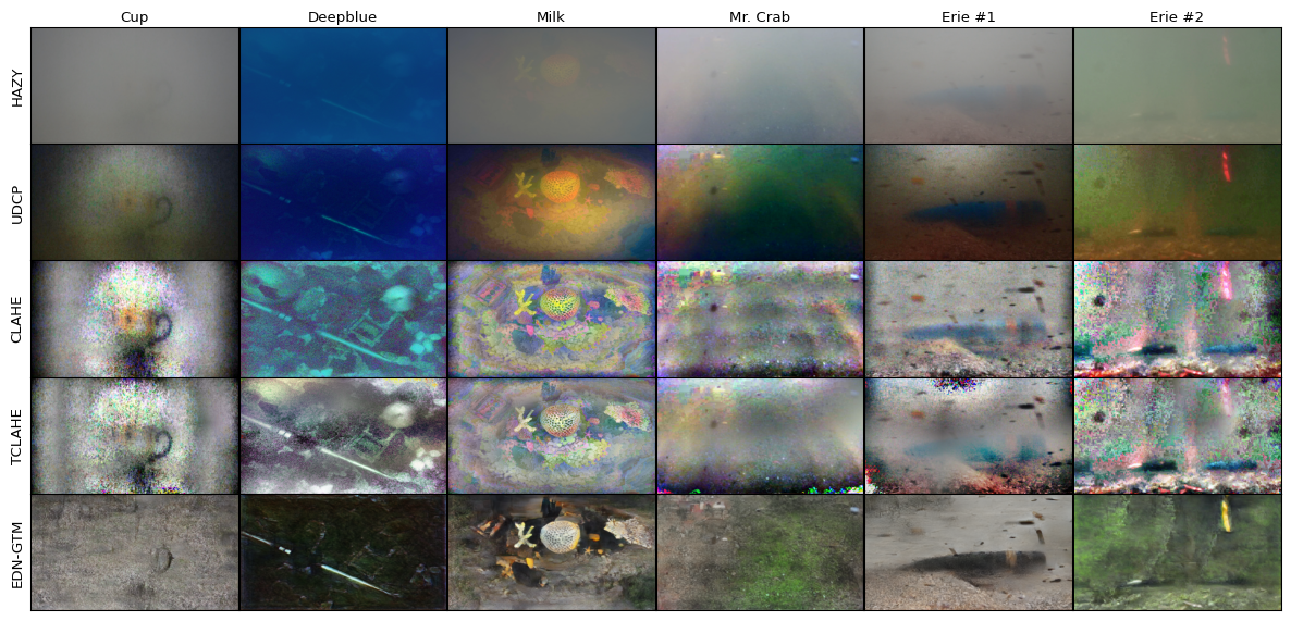
Sample outputs for UDCP (Underwater Dark Channel Prior; model-based), CLAHE (Contrast-Limit Adaptive Histogram Equalization; model-free), TCLAHE (Turbidity-Aware ibid; model-free), and EDN-GTM (Encoder-Decoder Network with Guided Transmission Map; learning). The first row holds the original hazy images. Images are taken from the underwater cup [1] and turbid (deepblue & milk) [2] datasets, as well as two videos of UXOs in lake Erie.